Frequency Domain Methods for Stability Analysis

8.1 Cauchy's Principle of the Argument

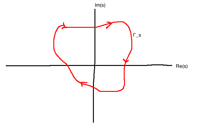
Consider a closed curve in the \(s\)-plane with no self-intersections and with negative (clockwise) orientation.

Now let \(G(s) \in \mathbb{R}(s)\). For each \(s \in \mathbb{C}\), \(G(s)\) is another complex number, so \(G: \mathbb{C} \rightarrow \mathbb{C}\)

If \(\Gamma_s\) doesn't pass through any poles of \(G\), then as \(s\) makes a circuit around \(\Gamma_s\), \(G(s)\) traces out a different closed curve that we'll call \(\Gamma_G\).

e.g. 8.1.1

\[G(s) = s-1\]

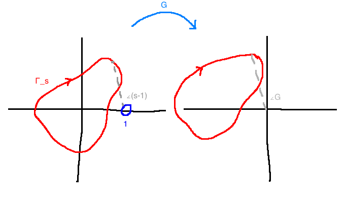
Since \(\Gamma_s\) encircles a zero of \(G\), the angle of \(G\) will change by \(-2\pi\) as \(s\) makes a circuit around \(\Gamma_s\).

e.g. 8.1.2

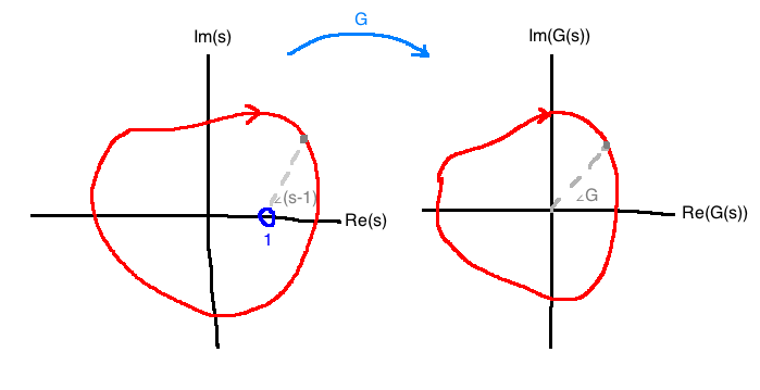
\[G(s) = s-1\]

Now the net change in \(\angle G(s)= \angle(s-1)\) as \(s\) moves around \(\Gamma_s\) is zero. This means that \(\Gamma_G\) does not encircle the origin.

e.g. 8.1.3

\[G(s) = \frac{1}{s-1}\]

\(\angle(s-a) = -\angle G\) because the pole is in the denominator.

Now, \(\angle (s-1)\) changes by \(-(-2\pi)=2\pi\) as the point makes a circuit aorund \(\Gamma_s\). Therefore, \(\Gamma_G\) must have a net angular change of \(2\pi\) as \(s\) moves around \(\Gamma_s\). \(\Gamma_G\) must encircle the origin once.

Theorem

Suppose \(G(s) \in \mathbb{R}(s)\) has no poles or zeroes on \(\Gamma_s\), but \(\Gamma_s\) encircles \(n\) poles of \(G\) and \(m\) zeroes of \(G\). Then, \(\Gamma_g\) has \(n-m\) counter-clockwise encirclements of the origin.

Proof

Write \(G\) like so:
\[G(s) = K \frac{\prod_i (s-z_i)}{\prod_i (s - p_i)}\]
\(K\) is a real gain, \(z_i\) are zeroes, and \(p_i\) are poles. Then, for each \(s\) on \(\Gamma_s\):
\[\angle G(s) = \angle K + \sum \angle(s-z_i) - \sum \angle (s-p_i)\]

If the zero \(z_i\) is enclosed by \(\Gamma_s\), the net change in the term \(\angle(s-z_i)\) after one circuit around \(\Gamma_s\) is \(-2\pi\). If \(z_i\) isn't enclosed, the net change is zero.

So, the net change in \(\angle G\) is \(m(-2\pi) - n(-2\pi) = (n-m)2\pi\).

\(\Gamma_G\) must encircle the origin \(n-m\) times in the counterclockwise direction.

Nyquist Contour

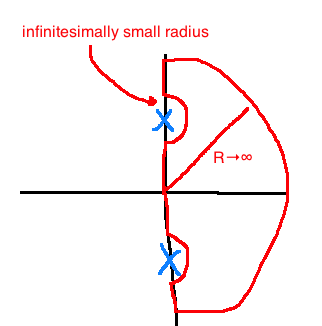
Take \(\Gamma_s\) to encircle the whole right-half plane

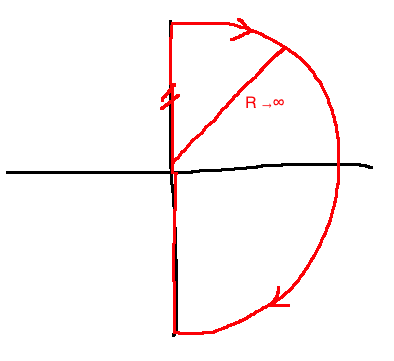
For this choice of \(\Gamma_S\), the corresponding curve \(\Gamma_G\) is called the Nyquist plot of \(G\). If \(G\) has no poles or zeroes on \(\Gamma_s\), then by the principle of the argument, the Nyquist plot will encircle the origin \(n-m\) times in counterclockwise direction.

\(n\) is the number of poles of \(G\) with \(\Re(s) \gt 0\), \(m\) is the number of zeroes of \(G\) with \(\Re(s) \gt 0\).

If \(G\) has poles on \(j\mathbb{R}\), we'll indent around them.

Nyquist stability criterion

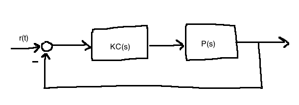
Assuming \(C,P\) are rational:

1. \(P,C\) are proper, \(CP\) strictly proper
2. No unstable pole-zero cancellations
3. \(K \ne 0\)

Key idea: if the system is IO stable, then the poles of \(\frac{Y(s)}{R(s)} = \frac{KC(s)P(s)}{1+KC(s)P(s)}\) must all be in \(\mathbb{C}^-\). So, we'll work with the transfer function \(G(s)=1+KC(s)P(s)\).

Theorem

Let \(n\) denote the number of poles of \(C(s)P(s)\) in \(\mathbb{C}^+\). Construct the Nyquist plot of \(C(s)P(s)\) indenting to the right around any poles on the imaginary axis. The feedback system is IO stable if and only if the Nyquist plot doesn't pass through \(\frac{-1}{K}\) and encircles \(\frac{-1}{K}\) exactly \(n\) times counterclockwise.

Proof

\[\frac{Y(s)}{R(s)} = \frac{KC(s)P(s)}{G(s)}\]
Since we've assumed no unstable pole-zero cancellations, IO stability is equivalent to \(G(s)\) having no zeroes with \(\Re(s) \ge 0\). (See Theorem 5.2.10.)

I.O. stability \(\Leftrightarrow \frac{KC(s)P(s)}{G(s)}\) has no poles with \(\Re(s) \ge 0 \Leftrightarrow G(s)\) has no zeroes with \(\Re(s) \ge 0\).

Since \(G(s)=1+K\frac{N_c(s)}{D_c(s)} \frac{N_p(s)}{D_p(s)} = \frac{D_cD_p+KN_cN_p}{D_cD_p}\), so \(G\) has the same poles as \(CP\). Therefore, \(G\) has \(n\) poles with \(\Re(s) \gt 0\).

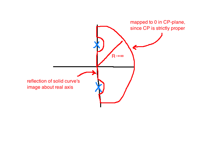
Since \(\Gamma_s\) indents around poles on \(j\mathbb{R}\) and since \(G\) is proper, \(\Gamma_s\) doesn't pass through any poles of \(G\). By the principle of the argument, \(\Gamma_G\) will encircle the origin \(n-m\) times in the counterclockwise direction.

Since we need no zeroes with \(\Re(s) \gt 0\), we need \(m=0\) for stability. Since \(C(s)P(s) = \frac{1}{K}G(s) - \frac{1}{K}\), the Nyquist plot of \(CP\) is going to be the Nyquist plot of \(G\) scaled (possibly by \(K\)) and then shifted to the left by \(\frac{-1}{K}\).

Conclusion: IO stability exists if and only if the Nyquist plot of \(CP\) encircles \(\frac{-1}{K}\) \(n\) times in the counterclockwise direction.

Remarks

Since \(C(s)P(s)\) is rational, we have:

• \(|C(j\omega)P(j\omega)| = |C(-j\omega)P(-j\omega)|\)
• \(\angle C(j\omega)P(j\omega) = -\angle C(-j\omega)P(-j\omega)\)
• So the image of \(\Gamma_s\) along the negative imaginary axis is a reflection about the real axis of the positive imaginary axis
• We see that a Nyquist plot is (aside from indentations) a polar plot of \(C(s)P(s)\). It's a plot of the curve \(\omega \rightarrow C(j\omega)P(j\omega)\) as \(\omega\) goes from 0 to \(\infty\)
• The Bode plot of \(C(s)P(s)\) is just \(20\log|C(j\omega)P(j\omega)|\) and \(\angle C(j\omega)P(j\omega)\) versus \(\log\omega\)

Procedure for applying the Nyquist criterion

Expect a question on the final asking to apply this

1. Pick \(\Gamma_s\) as the Nyquist contour, indenting to the right if necessary
2. Draw the image of \(\Gamma_s\) under the map \(C(s)P(s)\)
3. Observe \(N\), the number of counterclockwise encirclements of \(\frac{-1}{K}\) made by the Nyquist plot
4. Apply the Principle of the Argument:
   • \(N = n-m = \text{open loop poles in } \mathbb{C}^+ - \text{closed loop poles in } \mathbb{C}^+\)
   • \(n\) is known, \(m\) is unknown
5. We have input-output stability if and only if \(N = n\)

e.g.

\[C(s)P(s)=\frac{1}{s+10}\]

• On segment A, we have \(s=j\omega, \omega \in [0, \infty)\)
  • \(C(j\omega)P(j\omega)=\frac{1}{j\omega+10}=\frac{10-j\omega}{\omega^2+10^2}=\frac{10}{\omega^2+10}-\frac{j\omega}{\omega^2+10}\)
  • Start by finding the point that 0 translates to, and seeing what direction it goes when you increase \(\omega\)
  • Figure out where it crosses the imaginary axis, if at all
• Segment B: \(|s| = \infty\), so \(C(s)P(s) = 0\)
• Secment C is just a reflection of segment A
• Set \(K=1\) (for now) and observe the number \(N\) of counterclockwise encirclements of \(\frac{-1}{K}\) (\(N = 0\))
• \(N=n-m\), where in this case \(N=0, n=0\)
• Since \(N=n\), we have closed loop stability

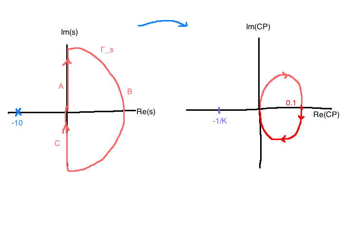
We can also test for other values of \(K\):

This implies it is stable for \(K \gt -10\).

e.g. comparing Nyquist to Bode

\[C(s)P(s) = \frac{1}{s+10}\]

• From Bode, when \(\omega \ll 1\), \(20\log|CP| \approx -20\), i.e. \(|CP| \approx 0.1\)
  • This is consistent with the Nyquist plot
• When \(\omega \ll 1\), \(\angle CP \approx 0^\circ\). Also consistent with Nyquist, which starts along the positive real axis.
• As \(\omega \rightarrow \infty\), \(20\log|CP| \rightarrow -\infty\), so \(|CP| \rightarrow 0\). This is consistent
• From Bode, \(\angle CP\) is always between \(-90^\circ\) and \(0^\circ\), which is consistent with the fact that Nyquist plot is always in quadrant 4.

e.g. 8.3.2

\[C(s)P(s) = \frac{s+1}{s(s-1)}\]

Segment A:

• \(s=j\omega\), \(\omega \in [\epsilon, \infty)\), \(0\lt\epsilon\lt 1\).
• \(C(j\omega)P(j\omega) = \frac{j\omega+1}{j\omega(j\omega-1)}=\frac{j-\omega}{\omega(1-j\omega)}=\frac{(j-\omega)(1+j\omega)}{\omega(1+\omega^2)}=\frac{-2}{1+\omega^2}+j\frac{1-\omega^2}{\omega(1+\omega^2)}\)
• When \(s = j\epsilon\), \(C(j\epsilon)P(j\epsilon) \approx -2 \underbrace{+}_\text{key!} j\infty\)
• When \(\omega=1\) (\(s=j\)), \(C(j)P(j)=-1+0j\)
• For all \(\omega \gt 1\), \(\Re(CP) \lt 0\) and \(\Im(CP) \lt 0\)

Segment B:

• \(|s|=\infty\), so \(|PC|=0\)

Segment C:

• Reflection of segment \(A\) about the real axis

Segment D:

• \(s=\epsilon e^{j\theta}\), \(\theta \in [-\frac{\pi}{2}, \frac{\pi}{2}]\)
• It's clear that \(|PC|=\infty\) along segment D.
• We want to know if it moves clockwise or counterclockwise as \(\theta\) goes from \(-\frac{\pi}{2}\) to \(\frac{\pi}{2}\)
• \(C(\epsilon e^{j\theta})P(\epsilon e^{j\theta}) = \frac{\epsilon e^{j\theta}+1}{\epsilon e^{j\theta}(\epsilon e^{j\theta}-1)} \approx \frac{1}{\epsilon e^{j\theta}(-1)} = \frac{-1}{\epsilon e^{j\theta}} = \frac{-\epsilon e^{-j\theta}}{\epsilon} = \frac{e^{j\pi} e^{-j\theta}}{\epsilon}=\frac{e^{j(\pi-\theta)}}{\epsilon}\)

Observe the number of counterclockwise encirclements of \(\frac{-1}{K}\):

Since we have \(n=1\), we need \(N=1\) for input-output stability. Therefore, \(K \gt 1\).

Stability margins, revisited

If a system is stable, how stable?

Phase margin

Nominal model: \(\phi=0\), input-output stability

How much phase change \(\phi\) can I tolerate before losing IO stability? Recall that \(|e^{j\phi}|=1\), \(\angle e^{j\phi}=\phi\)

e.g. 8.4.1

\[L(s) = \frac{1}{(s+1)^2}\]

\(n=0\), so we need zero counterclockwise encirclements of -1 to get IO stability.

• If we rotate the Nyquist plot by \(-\frac{\pi}{2}\), we get \(N=1\) and lose IO stability.
• Therefore the phase margin is around 90 degrees

Gain Margin

Nominal design: \(K=1\), IO stable. How much gain can we change \(K\) by before we lose stability?

e.g. 8.4.3

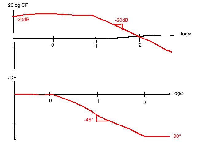
\[ L(s)=\frac{2}{(s+1)^2\left(\frac{s}{10}+1\right)}\]

\(n=0\) (no open-loop unstable poles), so we need \(N=0\) counterclockwise encirclements of -1 for IO stability.

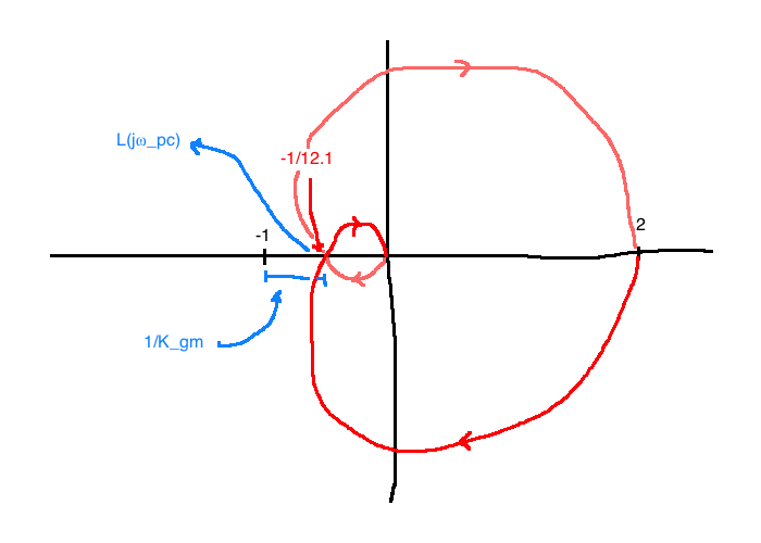
From the Nyquist criterion, the nominal model is IO stable. The system remains stable so long as \(\frac{-1}{K} \lt \frac{-1}{12.1}\). This means we can increase \(K\) up to 12.1 before losing stability. This value of \(K\) is called the gain margin.

Stability Margin

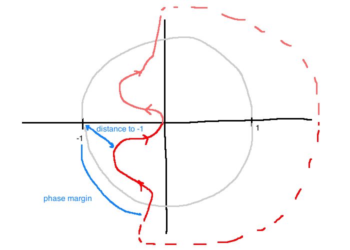
Phase margin is related to the distance on the Nyquist plot from to -1, measured as a rotation along the unit circle.

Gain margin is the distance on the Nyquist plot to -1 along the real axis.

More generally, we'll want to use the Euclidean distance from the Nyquist plot to -1 as a measure of stability.

e.g. 8.4.5

\[L(s) = \frac{0.38(s^2+0.1s+0.55)}{s(s+1)(s^2+0.06s+0.5)}\]

\(n=0\) so we need \(N=0\) counterclockwise encirclements of -1.

• good phase margin (\(\approx 70^\circ\))
• infinite gain margin (\(K_{gm}=\infty\))
• based on the above, we would conclude that the design is robust
• from the Nyquist plot we see that we're actually pretty close to encircling -1.

Consider for a moment our normal feedback system with no disturbances. The transfer function from \(r\) to \(e\):
\[\frac{E(s)}{R(s)} = \frac{1}{1+P(s)C(s)} =: S(s)\]

Assume IO stability. Then the distance from \(L=CP\) to -1 is:
\[\begin{align} \min_\omega \left|-1-L(j\omega)\right| &= \min_\omega \left|-1-CP\right|\\ &= \left(\max_\omega \left|\frac{1}{1+CP}\right|\right)^{-1}\\ &= \left(\max_\omega \left|S(j\omega)\right|\right)^{-1}\\ \end{align}\]

So, the distance from the Nyquist plot to -1 is the reciprocal of the peak magnitude of the Bode plot of \(S\). We'll call this \(S_m\), for stability margin.